The Kalman Filter Exposed

The Kalman filter sounds like one of those mysterious engineering spells whispered inside spacecraft, robots, financial models, and self-driving systems. In reality, it is not magic. It is a smart mathematical method for answering a very human question: “What is probably happening right now, even though my measurements are noisy, late, incomplete, or slightly wrong?”

That question appears everywhere. A phone tries to estimate your position while GPS bounces off buildings. A drone tries to stay level while wind, vibration, and cheap sensors argue with each other. A stock analyst tries to separate trend from market static. A spacecraft tries to know where it is when “close enough” is not exactly comforting. The Kalman filter helps by combining prediction, measurement, and uncertainty into one continuously updated estimate.

In plain English, the Kalman filter is a disciplined way to trust your model when your sensors are messy, trust your sensors when your model is drifting, and never trust anything blindly. It is the algorithmic equivalent of a calm engineer with a clipboard saying, “Interesting measurement, but let’s compare it with what physics expected.”

What Is the Kalman Filter?

The Kalman filter is an algorithm used to estimate the hidden state of a system over time. A “state” can be position, velocity, temperature, orientation, voltage, engine condition, or any variable that matters but cannot be measured perfectly. Instead of treating each measurement as truth, the filter asks how reliable the measurement is compared with the current prediction.

The classic Kalman filter works best with linear systems and Gaussian noise. “Linear” means the system can be described with equations that do not suddenly bend into chaos. “Gaussian noise” means the errors roughly follow the familiar bell-shaped curve. Those assumptions may sound strict, but they cover a surprising number of real-world problems. When they do not, engineers often use variations such as the Extended Kalman Filter or Unscented Kalman Filter.

At its heart, the Kalman filter runs a two-step loop: predict and update. First, it predicts where the system should be based on the previous estimate and a model of how the system moves. Then it updates that prediction using the newest measurement. The final estimate lands somewhere between the prediction and the measurement, depending on which one is more trustworthy.

The Big Idea: Predict, Measure, Correct

Imagine tracking a train moving along a straight track. You know its last position and speed. Based on that, you can predict where it should be two seconds later. But your sensor reports a slightly different position because sensors are imperfect little gremlins. Should you believe the prediction or the sensor?

The Kalman filter says: believe both, but not equally. If the sensor is known to be accurate, the filter moves the estimate closer to the measurement. If the sensor is noisy, the filter leans more heavily on the prediction. This balancing act is controlled by the Kalman gain, which decides how aggressively the estimate should respond to new measurements.

This is why the filter is so powerful. It does not simply smooth data after the fact. It uses a model of the system and updates that model in real time. It is both predictive and corrective, like a weather forecast that actually listens when rain starts hitting the window.

The Core Parts of a Kalman Filter

1. The State Estimate

The state estimate is the filter’s best guess about the system right now. In a moving car example, the state might include position and velocity. In a drone, it might include angle, angular velocity, altitude, and acceleration. The filter does not need to directly measure every state variable. Sometimes it can infer hidden variables from related measurements.

2. The Process Model

The process model describes how the system changes from one moment to the next. For a vehicle, this might involve equations of motion. For an economic signal, it might describe how a trend evolves. The model is useful, but never perfect. Tires slip, engines vibrate, markets panic, and reality enjoys improvisation.

3. Measurement Data

Measurements come from sensors, observations, or input data. They might include GPS coordinates, radar distance, gyroscope readings, temperature values, or noisy financial indicators. The Kalman filter uses these measurements to correct its prediction.

4. Uncertainty

Uncertainty is the secret sauce. The filter keeps track of how confident it is in its own estimate. This confidence is represented with covariance, which measures how much error is expected. If uncertainty grows, the filter becomes more willing to listen to measurements. If uncertainty shrinks, it becomes more confident in its predictions.

5. The Kalman Gain

The Kalman gain determines how much the new measurement changes the estimate. A high gain means the filter strongly follows measurements. A low gain means it trusts the prediction more. When tuned properly, this makes the filter responsive without becoming jumpy.

Why the Kalman Filter Matters

The Kalman filter became famous because it works beautifully in problems where decisions must be made continuously under uncertainty. It has been used in aerospace navigation, tracking systems, control engineering, robotics, signal processing, economics, computer vision, and many other fields. Its historical connection with spacecraft navigation helped make it legendary, but its everyday usefulness is just as impressive.

Modern systems are packed with sensors, but more sensors do not automatically mean better truth. In fact, more sensors can mean more disagreement. GPS may say one thing, an accelerometer another, and a gyroscope may slowly drift like it is telling a ghost story. The Kalman filter provides a framework for sensor fusion, combining multiple noisy inputs into a more stable estimate.

Real-World Examples of Kalman Filtering

GPS and Smartphone Navigation

Your phone does not simply accept every GPS reading as perfect. GPS can be noisy, especially near tall buildings, indoors, or under tree cover. A Kalman-style estimator can combine GPS with accelerometer and gyroscope data to produce smoother movement and more realistic position estimates. Without filtering, your blue dot might behave like it had too much coffee.

Robotics and Autonomous Vehicles

Robots need to know where they are, where they are going, and how fast they are moving. Wheel encoders can drift. Cameras can lose features. Lidar can be confused by reflective surfaces. IMUs accumulate error over time. A Kalman filter or one of its nonlinear relatives can fuse these signals to estimate position, velocity, and orientation more reliably.

Aerospace and Navigation

Aircraft and spacecraft depend on accurate state estimation. Navigation systems combine inertial measurements, radar, radio signals, star trackers, or other data sources to estimate trajectory and attitude. In these environments, filtering is not a luxury. It is part of making complex motion understandable and controllable.

Finance and Time-Series Analysis

In finance and economics, state-space models and Kalman filtering can estimate hidden trends, changing volatility, or unobserved components in time-series data. The idea is not that the filter predicts markets with crystal-ball certainty. Sadly, there is no “retire by Friday” button. Instead, it helps separate signal from noise when the underlying state changes over time.

Computer Vision and Object Tracking

In video tracking, the Kalman filter can estimate where an object will appear in the next frame. If a camera briefly loses sight of the object, the prediction step can keep the tracker alive for a short time. When the object reappears, the update step corrects the estimate. This is useful in surveillance, sports analytics, augmented reality, and motion capture.

The Math Without the Migraine

The Kalman filter has a reputation for mathematical intimidation. Matrices appear. Covariances multiply. Transposes enter the room wearing sunglasses. But the concept is easier than the notation suggests.

Think of the filter as maintaining two things: an estimate and a confidence level. At every time step, it predicts the next estimate and predicts how uncertain that estimate has become. Then it compares the actual measurement with the predicted measurement. The difference is called the innovation or residual. If the measurement surprises the filter, the innovation is large. If the measurement matches expectations, the innovation is small.

The filter then adjusts the estimate based on the innovation and Kalman gain. After the adjustment, it updates its uncertainty. This cycle repeats again and again. No need to store every past measurement; the filter is recursive, meaning the current estimate already summarizes what it learned before.

Why “Recursive” Is a Big Deal

A recursive algorithm updates itself using only the previous result and the latest input. That makes the Kalman filter efficient for real-time systems. A drone cannot pause midair to reread every sensor measurement since takeoff. A spacecraft cannot say, “Give me a minute, I’m recalculating my entire childhood.”

Because the Kalman filter only needs the previous state estimate, previous uncertainty, current model, and current measurement, it can run quickly on embedded systems. This efficiency is one reason it became so popular in control systems and navigation.

Common Types of Kalman Filters

Standard Kalman Filter

The standard Kalman filter is designed for linear systems. It is elegant, efficient, and mathematically optimal under the right assumptions. If your system can be modeled linearly and your noise behaves nicely, this is the classic tool.

Extended Kalman Filter

The Extended Kalman Filter, often called EKF, handles nonlinear systems by approximating them locally with linear equations. It uses Jacobian matrices to describe how the system changes around the current estimate. EKF is widely used in robotics, navigation, and sensor fusion, but it can become unstable if the system is highly nonlinear or poorly modeled.

Unscented Kalman Filter

The Unscented Kalman Filter, or UKF, handles nonlinear systems differently. Instead of linearizing with derivatives, it selects a set of representative points called sigma points, pushes them through the nonlinear model, and reconstructs the estimate. UKF can perform better than EKF in some nonlinear problems, especially when calculating Jacobians is painful.

Ensemble Kalman Filter

The Ensemble Kalman Filter uses a group of sample states to represent uncertainty. It is especially useful in very large systems, such as weather prediction and geophysical modeling, where directly storing huge covariance matrices would be impractical.

Where Beginners Usually Go Wrong

The first beginner mistake is thinking the Kalman filter is a magic noise remover. It is not. If the model is bad, the measurements are misunderstood, or the uncertainty values are nonsense, the filter can confidently produce polished garbage. Very smooth garbage, perhaps, but garbage with excellent posture.

The second mistake is tuning the process noise and measurement noise carelessly. Process noise describes how much uncertainty exists in the model. Measurement noise describes how much uncertainty exists in the sensor. If measurement noise is set too low, the filter may chase noisy readings. If process noise is set too low, it may ignore real changes. Good tuning is often the difference between a brilliant filter and a stubborn one.

The third mistake is ignoring units and coordinate systems. Mixing meters with centimeters, degrees with radians, or local coordinates with global coordinates can produce wild results. The Kalman filter will not politely raise its hand and say, “Excuse me, your coordinate frame is a disaster.” It will simply fail in mathematically creative ways.

How to Think About Tuning

Tuning a Kalman filter is part science, part engineering judgment, and part patient debugging. Start with the real sensor specifications when available. Estimate measurement noise from repeated measurements under stable conditions. Estimate process noise based on how unpredictable the system truly is.

If the filtered output is too jittery, the filter may be trusting measurements too much. If the output lags behind real motion, it may be trusting the model too much. The goal is not maximum smoothness. The goal is accurate estimation with appropriate responsiveness.

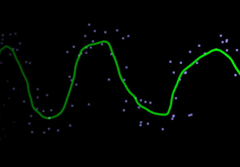
The Kalman Filter Versus Simple Moving Average

A moving average smooths data by averaging recent values. It is simple and useful, but it does not understand the system. It does not know whether an object has velocity, acceleration, or physical constraints. It simply blends numbers.

The Kalman filter is more intelligent because it uses a model. It can estimate hidden variables, predict future states, and combine different kinds of measurements. A moving average may smooth a position signal. A Kalman filter may estimate both position and velocity from noisy position measurements. That is a much bigger trick.

When Not to Use a Kalman Filter

The Kalman filter is powerful, but it is not always the right tool. If the data is simple and offline, a basic smoothing method may be enough. If the system is extremely nonlinear and non-Gaussian, particle filters or other Bayesian methods may work better. If the model is unknown or changes dramatically, machine learning or adaptive filtering may be more suitable.

Use a Kalman filter when you have a system model, sequential measurements, uncertainty, and a need for real-time estimation. Do not use it just because it sounds impressive in a meeting. Although, to be fair, saying “we implemented a recursive Bayesian estimator” does make the coffee taste more expensive.

Experience-Based Insights: What Working With Kalman Filters Teaches You

The first experience most people have with a Kalman filter is confusion. The equations look clean in textbooks, but implementation quickly reveals practical questions. What should the initial covariance be? How noisy is the sensor, really? Is the model too simple? Why does the estimate explode after three seconds? Why did changing one tiny matrix value make the output look like a seismograph during a dinosaur parade?

One useful lesson is to begin with the simplest possible model. For example, if you are tracking one-dimensional motion, start with position and velocity. Use synthetic data first, where the true answer is known. Add controlled noise. Check whether the filter recovers the hidden state. This prevents you from debugging math, sensors, code, and reality all at the same time.

Another practical lesson is that visualization matters. Plot the raw measurement, prediction, filtered estimate, and true value if available. Many Kalman filter problems become obvious when plotted. If the estimate follows the measurement too closely, measurement noise may be underestimated. If it reacts too slowly, process noise may be underestimated. If it drifts away entirely, the model or measurement matrix may be wrong.

Working with real sensors also teaches humility. Sensor datasheets are helpful, but actual sensor behavior depends on temperature, vibration, mounting, calibration, sampling rate, and environment. An IMU on a quiet desk behaves differently from an IMU on a vibrating robot. GPS in an open field behaves differently from GPS in a city street. A good Kalman filter respects these differences through realistic noise modeling.

In robotics, one common experience is discovering that sensor fusion is not simply “throw all sensors into the filter and celebrate.” Each sensor measures something specific, at a specific rate, in a specific coordinate frame, with specific delays and errors. The filter must be designed around those realities. A slow GPS update and a fast IMU update can work beautifully together, but only if timing and measurement models are handled carefully.

Another valuable experience is learning that the best filter is not always the most complicated one. Beginners often jump from the standard Kalman filter to EKF, UKF, or particle filters before fully understanding the problem. Sometimes a linear model with careful tuning performs better than a fancy nonlinear filter with poor assumptions. Engineering is not about using the most advanced tool; it is about using the right tool without making the system cry.

Debugging Kalman filters also builds strong habits. You learn to check dimensions, units, timestamps, and coordinate transformations. You learn to separate prediction errors from measurement errors. You learn that a stable estimate is not automatically a correct estimate. You learn that uncertainty is not a decorative matrix; it is the filter’s opinion about how wrong it might be.

Perhaps the most important experience is realizing that Kalman filtering is a way of thinking, not just an algorithm. It teaches you to combine prior knowledge with new evidence. It teaches you to quantify trust. It teaches you to update beliefs without panicking every time a noisy measurement appears. That mindset applies far beyond robotics or aerospace. It is useful in analytics, forecasting, decision-making, and everyday reasoning.

The Kalman filter is exposed, then, not as a mysterious black box but as a practical philosophy: predict carefully, measure skeptically, correct intelligently, and repeat. It is not perfect. It depends on assumptions. It needs tuning. It can fail spectacularly when misused. But when matched to the right problem, it turns noisy streams of data into clear, actionable estimates. That is why, decades after its introduction, it still sits quietly inside some of the most sophisticated systems humans build.

Conclusion

The Kalman filter remains one of the most useful algorithms in estimation, tracking, navigation, and sensor fusion. Its brilliance lies in its balance: it respects mathematical models without worshiping them, listens to measurements without blindly obeying them, and constantly updates uncertainty as new information arrives.

For developers, engineers, analysts, and curious learners, understanding the Kalman filter opens the door to better thinking about noisy data. Whether you are smoothing GPS signals, tracking a robot, modeling time-series data, or simply trying to understand how machines make sense of uncertainty, the Kalman filter is worth learning. It is not just a filter. It is a disciplined conversation between prediction and evidence.